Updated November 23, 2020

This session

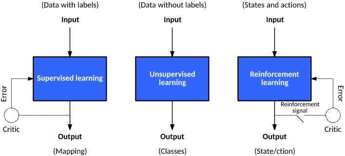
Welcome all to this introduction to machine learning (ML). In this session we will:

  1. Introduce to the general logic of machine learning
  2. How to generalize?
  3. The Bias-Variance Tradeoff
  4. Selecting and tuning ML models

Introduction

What is ML?

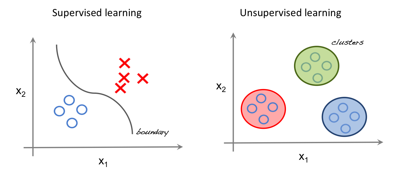
As with any concept, machine learning may have a slightly different definition, depending on whom you ask. A little compilation of definitions by academics and practioneers alike:

  • “Machine Learning at its most basic is the practice of using algorithms to parse data, learn from it, and then make a determination or prediction about something in the world.” - Nvidia
  • “Machine learning is the science of getting computers to act without being explicitly programmed.” - Stanford
  • “Machine learning is based on algorithms that can learn from data without relying on rules-based programming.”- McKinsey & Co.
  • “Machine learning algorithms can figure out how to perform important tasks by generalizing from examples.” - University of Washington
  • “The field of Machine Learning seeks to answer the question”How can we build computer systems that automatically improve with experience, and what are the fundamental laws that govern all learning processes?" - Carnegie Mellon University

Supervised vs. Unsupervised ML

Unsupervised ML

Tasks related to pattern recognition and data exploration, in dase there yet does not exist a right answer or problem structure. Main application

  1. Dimensionality reduction: Finding patterns in the features of the data
  2. Clustering: Finding homogenous subgroups within larger group

Supervised ML

  • Concerned with labeling/classification/input-output-mapping/prediction tasks
  • Subject of the next lecture, so stay patient

This is what is currently driving >90% ML applications in research, industry, and policy, and will be the focus on the following sessions.

Supervised vs. Unsupervised ML: Intuitive

  • Unsupervised ML: Finding ex-ante undefined pattern in data.
  • Sypervised ML: Predicting well defined outcome of interest.

Supervised vs. Unsupervised ML: Functional

  • Unsupervised ML: Creating formerly undefind labels.
  • Sypervised ML: MApping input to output.

Contrasting ML with inferential statistics

Inferential Statistics

  • Mostly interested in producing good parameter estimates: Construct models with unbiased estimates of \(\beta\), capturing the relationship \(x\) and \(y\).
  • Supposedly models: Causal effect of directionality \(x \rightarrow y\), robust across a variety of observed as well as up to now unobserved settings.
  • How: Carefully draw from theories and empirical findings, apply logical reasoning to formulate hypotheses.
  • Typically, multivariate testing, cetris paribus.
  • Main concern: Minimize standard errors \(\epsilon\) of \(\beta\) estimates.
  • Not overly concerned with overall predictive power (eg. \(R^2\)) of those models, but about various type of endogeneity issues, leading us to develop sophisticated identification strategies

ML Approach

  • To large extend driven by the needs of the private sector \(\rightarrow\) data analysis is gear towards producing good predictions of outcomes \(\rightarrow\) fits for \(\hat{y}\), not \(\hat{\beta}\)
    • Recommender systems: Amazon, Netflix, Sportify ect.
    • Risk scores: Eg.g likelihood that a particular person has an accident, turns sick, or defaults on their credit.
    • Image classification: Finding Cats & Dogs online
    • Predictive policing
  • Often rely on big data (N,\(x_i\))
  • Not overly concerned with the properties of parameter estimates, but very rigorous in optimizing the overall prediction accuracy.
  • Often more flexibility wrt. the functional form, and non-parametric approaches.
  • No “build-in”" causality guarantee \(\rightarrow\) verification techniques.
  • Often sporadically used in econometric procedures, but seen as “son of a lesser god”.

Statistics Refresher

Introduction to regression problems

Lets for a second recap linear regression techniques, foremost the common allrounder and workhorse of statistical research since some 100 years.

OLS Basic Properties

  • Outcome: contionous
  • Predictors: continous, dichotonomous, categorical
  • When to use: Predicting a phenomenon that scales and can be measured continuously

Functional form

\[y = \beta_0 + \beta_1 x_1 + \beta_2 x_2 + ... + \beta_n x_n + \epsilon \]

  • \(y\) = Outcome, \(x_i\) = observed value \(ID_i\)
  • \(\beta_0\) = Constant
  • \(\beta_i\) = Estimated effect of \(x_i\) on \(y\) , slope of the linear function
  • \(\epsilon\) = Error term

  • Just imagine some data.

  • OLS will just fit a straight line through your data.

  • OLS minimizes the sum of (squared) errors between our prediction-line and the observed outcome.

Regression Example

  • We generate some data, where \(y\) is a linear function of \(x\) plus random noise.

Dependent variable:
y
x 0.304***
(0.008)
Constant 14.792***
(0.453)
Observations 500
Log Likelihood -1,526.330
Akaike Inf. Crit. 3,056.661
Note: p<0.1; p<0.05; p<0.01


  • We can now fit a linear regression model that aims at discovering the underlying relationship.

  • We can also visualize that
  • We again see the model puts a straight line through our data
  • This line tells us how to predict the outcome y based on observed values of x
  • The coeffficient indicates the slope of this linear function.

Prediction based on fitted model

* After the model’s parameters are fitted, we can use it to predict our outcome of interest. * Is here done on the same data, but obviously in most cases more relevant on new data.

Assesing predictive power of the model

  • So, how well does our model now predict?
  • A common measure of predictive power of regressions models is the Root-Mean-Squared-Error (RSME), calculate as follows:

\[ RMSE = \sqrt{\frac{1}{n}\Sigma_{i=1}^{n}{\Big(y_i - \hat{y_i} \Big)^2}}\]

Keep in mind, this root&squared thingy does nothing with the error term except of transforming negative to positive values.

## [1] 5.112672

  • We can also visualize the error term
  • Appears to be rather normally distributed.

Introduction to classification problems

## # A tibble: 6 x 2
##        x     y
##    <dbl> <int>
## 1  1.33      1
## 2  1.43      1
## 3 -1.73      0
## 4 -1.24      0
## 5  0.196     1
## 6 -1.03      0
  • Lets assume our outcome of interest is categorigal (Yes/No, Class1/Class2/Class3…)

  • This is how it looks like.

  • We can obviously fit a linear model on it, but what do the predicted values mean then?
  • We could intrpet them as probability: y=TRUE
  • However, how does the model fit the data?

  • I guess we would like more to have something like this below, right?
  • This seems to be more suited for class prediction, right?

Dependent variable:
y
x 4.977***
(0.489)
Constant -0.085
(0.170)
Observations 500
Log Likelihood -113.223
Akaike Inf. Crit. 230.447
Note: p<0.1; p<0.05; p<0.01
  • How do we do that?
  • The easiest way is to use a glm, where we just change the distribution from gaussian to binomial

  • Based on this model we can now also carry out predictions

Model metrics for classification problems

The Confusion matrix

Confussion Matrix Unpacked

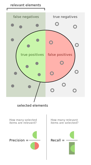
It is the 2x2 matrix with the following cells:

  • True Positive: (TP): You predicted positive and it’s true.

  • True Negative: (TN)

    • Interpretation: You predicted negative and it’s true.
    • You predicted that a man is not pregnant and he actually is not.
  • False Positive: (FP) - (Type 1 Error): You predicted positive and it’s false.

  • False Negative: (FN) - (Type 2 Error): You predicted negative and it’s false.

  • Just remember, We describe predicted values as Positive and Negative and actual values as True and False.

  • Out of combinations of these values, we dan derive a set of different quality measures.

  • The simplest one is the models accuracy, the share of correct predictions in all predictions

Accuracy (ACC)

\[ {ACC} ={\frac {\mathrm {TP} + \mathrm {TN} }{P+N}} \]

Summary of Metrics

Sensitivity also called recall, hit rate, or true positive rate (TPR) \[ {TPR} ={\frac {\mathrm {TP} }{P}}={\frac {\mathrm {TP} }{\mathrm {TP} +\mathrm {FN} }}\]

Specificity, also called selectivity or true negative rate (TNR) \[ {TNR} ={\frac {\mathrm {TN} }{N}}={\frac {\mathrm {TN} }{\mathrm {TN} +\mathrm {FP} }}\]

Precision, also called positive predictive value (PPV) \[ {PPV} ={\frac {\mathrm {TP} }{\mathrm {TP} +\mathrm {FP} }} \]

F1 score: weighted average of the true positive rate (recall) and precision. \[ F_{1}={\frac {2\mathrm {TP} }{2\mathrm {TP} +\mathrm {FP} +\mathrm {FN} }} \]

Creating a confusion matrix

  1. Put real and predicted values side-by-side
  2. Aggregate on Truth-Prediction level
  3. Create the confusion matrix and calculate th corresponding values

ROC and AUC

  • An ROC curve is a derivative of the confusion matrix and predicted class-probabilities.
  • The curve plots true positive rate (sensitivity) against the false positives rate (1-specificity)
  • The area-under-the-curve (AUC) also good and balanced indicator of a models predictive power.

Generalization in ML models

Generalization via “Out-of-Sample-Testing”

  • With so much freedom wrt. feature selection, functional form ect., models are prone to over-fitting. And no constraints by asymptotic properties, causality and so forth, how can we generalize anything?
  • In ML, generalization is not achived by statistical derivatives and theoretical argumentation, but rather by answering the practical question: How well would my model perform with new data? To answer this question, Out-of-Sample-Testing is usually taken as solution. Here, you do the following
  1. Split the dataset in a training and a test sample.
  2. Fit you regression (train your model) on one dataset
    • Optimal: Tune hyperparameters by minimizing loss in a validation set.
    • Optimal: Retrain final model configuration on whole training set
  3. Finally, evaluate predictive power on test sample, on which model is not fitted.

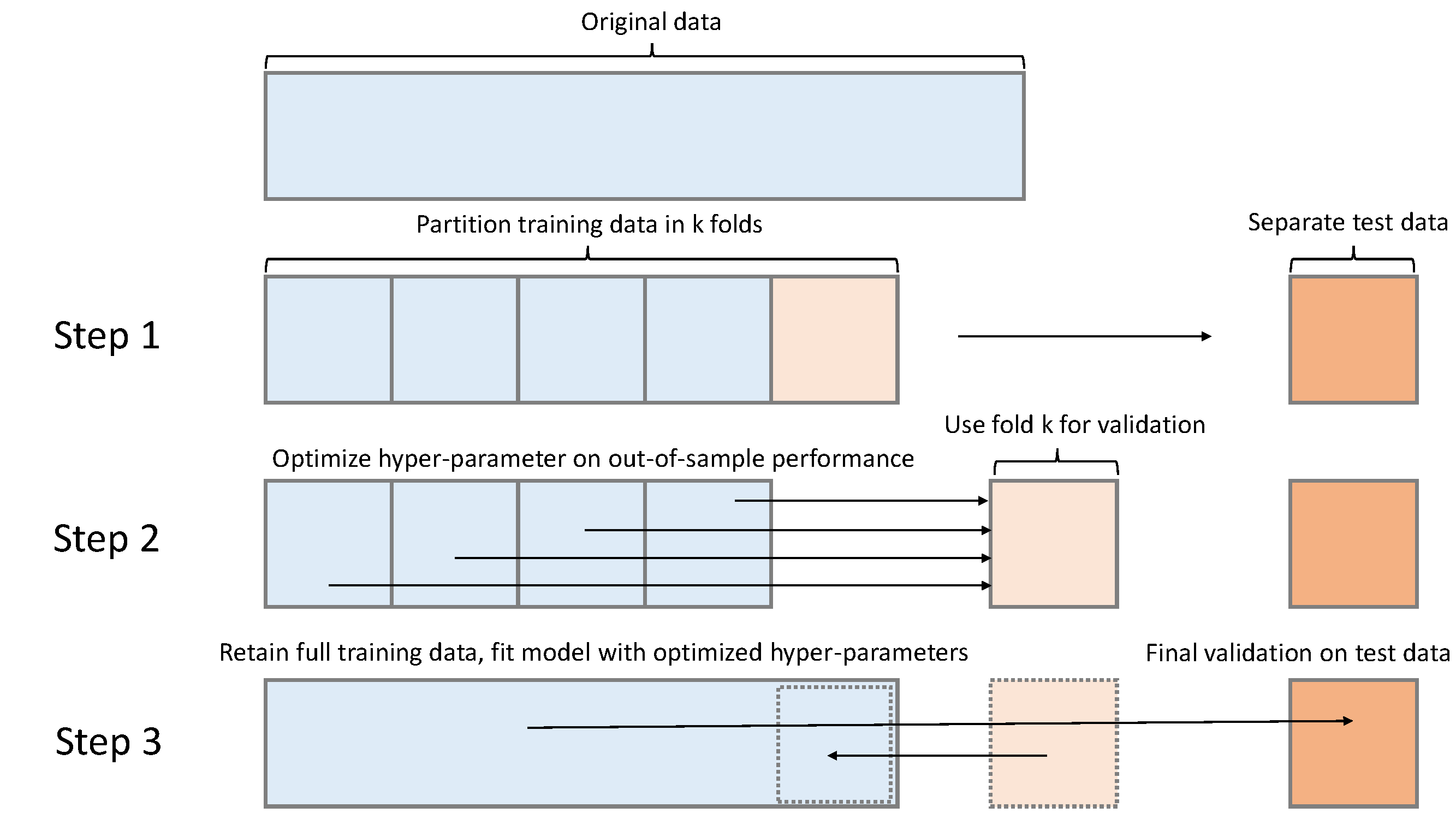
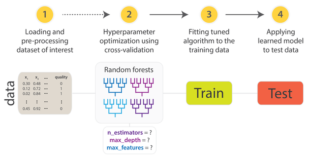
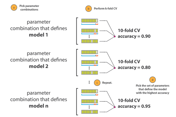
An advanced version is a N-fold-Crossvalidation, where this process is repeated several time during the hyperparameter-tuning phase.

N-fold-Crossvalidation

Bias-Variance Tradeoff

  • As a rule-of-thumb: Richer and more complex functional forms and algorithms tend to be better in predictign complex real world pattern.
  • This is particularly true for high-dimensional (big) data.
  • However, flexible algorithms at one point become so good in mimicing the pattern in our data that they overfit.
  • Overfitted algorithms are to much tuned towards a specific dataset and might not reproduce the same accuracy in new data.

Bias-Variance Tradeoff

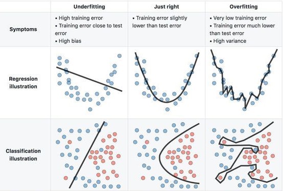
Generally, we call this tension the bias-variance tradeoff, which we can decompose in the two components:

  1. Bias Error The simplifying assumptions made by a model to make the target function easier to learn. Generally, simple parametric algorithms have a high bias making them fast to learn and easier to understand but generally less flexible.
  2. Variance Error: Variance is the amount that the estimate of the target function will change if different data was used. Ideally, it should not change too much from one training dataset to the next, meaning that the algorithm is good at picking out the hidden underlying mapping between the inputs and the output variables.
  • As a result, the predictive performance (on new data) of algorithms and models will always depend on this trade-off between bias and variance. Mathematically, this can be formalized as:

\[{\displaystyle \operatorname {E} {\Big [}{\big (}y-{\hat {f}}(x){\big )}^{2}{\Big ]}={\Big (}\operatorname {Bias} {\big [}{\hat {f}}(x){\big ]}{\Big )}^{2}+\operatorname {Var} {\big [}{\hat {f}}(x){\big ]}+\sigma ^{2}}\]

Note:

  • Bias and variance are reducible errors which decline when using a more suitable model to model the underlying relationships in the data
  • \(\sigma^2\) denotes the unreducible complexity caused by random noise, measurement errors, or missing variables, which represent a boundary to our ability to predict given the data at hand.

Example

  • We create some data, where \(x\) is a uniformly distributed random variable bounded between 0-1, and \(y = sin(n)\)

Example

  • We add some random noise, which is normally distributed

Fitting different models

  • We see the formerly clearly visible underlying relationship between \(x\) and \(y\) now to some extent disturbed by this noise.
  • However, keep in mind that the process that generated the data is still \(y = sinus(x)\)
  • This would also be the best funtional form to identify by any predictive algorithm.

Lets see how models with different levels of complexity would interpret the reælationship between \(x\) and \(y\):

  1. \(y\) is modeled as a linear function of \(x\)
  2. \(y\) is modeled as a curvelinear function of \(x\)
  3. \(y\) is modeled as a compex polynomial function of \(x\)

Regularization

  • The process of minimizing bias and variance errors is called regularization (inpractice also refered to as hyperparameter-tuning)
  • We aim at selecting the right model class, functional form, and degree of complexity to jointly minimize in-sample loss but also between-sample variations.

Mathematically speaking, we try to minimize a loss function \(L(.)\) (eg. RMSE) the following problem:

\[minimize \underbrace{\sum_{i=1}^{n}L(f(x_i),y_i),}_{in-sample~loss} ~ over \overbrace{~ f \in F ~}^{function~class} subject~to \underbrace{~ R(f) \leq c.}_{complexity~restriction}\]

Hyperparameter Tuning

  • Most model classes have parameters influencing their functionality
  • These parameters often influence predictive performance of models
  • Finding the right hyperparameter configuration (tuning) is therefore an essiential part when engineering predictive algorithms

Tune Grids

Examples of Model classes

Popular model classes

Elastic Net

The elastic net has the functional form of a generalized linear model, plus an adittional term \(\lambda\) a parameter which penalizes the coefficient by its contribution to the models loss in the form of:

\[\lambda \sum_{p=1}^{P} [ 1 - \alpha |\beta_p| + \alpha |\beta_p|^2]\]

  • Here, we have 2 tunable parameters, \(\lambda\) and \(\alpha\). If \(\alpha = 0\), we are left with \(|\beta_i|\), turning it to a lately among econometricians very popular Least Absolute Shrinkage and Selection Operator (LASSO) regression.
  • Obviously, when \(\lambda = 0\), the whole term vanishes, and we are again left with a generalized linear model.

Decision Trees

  • Mostly used in classification problems on continuous or categorical variables.
  • Idea: split the population or sample into two or more homogeneous sets (or sub-populations) based on most significant splitter / differentiator in input variables.
  • Repeat till stop criterium reachesd. leads to a tree-like structure.

This class became increasingly popular in business and other applications. Some reasons are:

  • Easy to Understand: Decision tree output is very easy to understand even for people from non-analytical background.
  • Useful in Data exploration: Decision tree is one of the fastest way to identify most significant variables and relation between two or more variables.
  • Data type is not a constraint: It can handle both numerical and categorical variables.
  • Non Parametric Method: Decision tree is considered to be a non-parametric method. This means that decision trees have no assumptions about the space distribution and the classifier structure.

Some tree terminology

  • Root Node: Entire population or sample and this further gets divided into two or more homogeneous sets.
  • Splitting: It is a process of dividing a node into two or more sub-nodes.
  • Decision Node: When a sub-node splits into further sub-nodes, then it is called decision node.
  • Leaf/ Terminal Node: Nodes do not split is called Leaf or Terminal node.

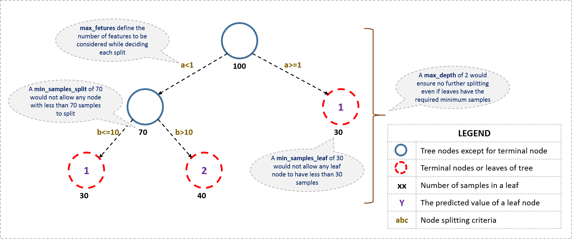
The decision of making strategic splits heavily affects a tree’s accuracy. So, How does the tree decide to split? This is different across the large family of tree-like models. Common approaches:

  • Gini Index
  • \(\chi^2\)
  • Reduction in \(\sigma^2\)

Some common complexity restrictions are:

  • Minimum samples for a node split
  • Minimum samples for a terminal node (leaf)
  • Maximum depth of tree (vertical depth)
  • Maximum number of terminal nodes
  • Maximum features to consider for split

Likewise, there are a variety of tunable hyperparameters across different applications of this model family.

Random Forest

  • As a continuation of tree-based classification methods, random forests aim at reducing overfitting by introducing randomness via bootstrapping, boosting, and ensemble techniques.
  • It is a type of ensemble learning method, where a group of weak models combine to form a powerful model.
  • The idea here is to create an “ensemble of classification trees”", all grown out of a different bootstrap sample. Having grown a forest of trees, every tree performs a prediction, and the final model prediction is formed by a majority vote of all trees.
  • This idea close to Monte Carlo simulation approaches, tapping in the power of randomness.

Summing up

What we covered so far

In this session, took a look at

  • What is ML to start with?
  • The difference between traditional inferential statistics and ML
  • Out-of-Sample validation
  • The Bias-Variance Tradeoff
  • How to tune ML models
  • ML model classes

In the next sessions, we will apply what we learned so far… so stay tuned!